If you’re looking to enhance your content understanding and search capabilities, audio embeddings offer a powerful solution. In this post, you’ll learn how to use Amazon Nova Multimodal Embeddings to transform your audio content to searchable, intelligent data that captures acoustic features like tone, emotion, musical characteristics, and environmental sounds.

Finding specific content in these libraries presents real technical challenges. Traditional search methods like manual transcription, metadata tagging, and speech-to-text conversion work well for capturing and searching spoken words. However, these text-based approaches focus on linguistic content rather than acoustic properties like tone, emotion, musical characteristics, and environmental sounds. Audio embeddings address this gap. They represent your audio as dense numerical vectors in high-dimensional space that encode both semantic and acoustic properties. These representations let you perform semantic search using natural language queries, match similar-sounding audio, and automatically categorize content based on what it sounds like rather than just metadata tags. Amazon Nova Multimodal Embeddings, announced on October 28, 2025, is a multimodal embedding model available in Amazon Bedrock [1]. It’s the unified embedding model that supports text, documents, images, video, and audio through a single model for cross-modal retrieval with accuracy.

This post walks you through understanding audio embeddings, implementing Amazon Nova Multimodal Embeddings, and building a practical search system for your audio content. You’ll learn how embeddings represent audio as vectors, explore the technical capabilities of Amazon Nova, and see hands-on code examples for indexing and querying your audio libraries. By the end, you’ll have the knowledge to deploy production-ready audio search capabilities.

Understanding Audio Embeddings: Core Concepts

Vector Representations for Audio Content

Think of audio embeddings as a coordinate system for sound. Just as GPS coordinates pinpoint locations on Earth, embeddings map your audio content to specific points in high-dimensional space. Amazon Nova Multimodal Embeddings gives you four-dimension options: 3,072 (default), 1,024, 384, or 256 [1]. Each embedding is a float32 array. Individual dimensions encode acoustic and semantic features—rhythm, pitch, timbre, emotional tone, and semantic meaning—all learned through the model’s neural network architecture during training. Amazon Nova uses Matryoshka Representation Learning (MRL), a technique that structures embeddings hierarchically [1]. Think of MRL like Russian nesting dolls. A 3,072-dimension embedding contains all the information, but you can extract just the first 256 dimensions and still get accurate results. Generate embeddings once, then choose the size that balances accuracy with storage costs. No need to reprocess your audio when trying different dimensions— the hierarchical structure lets you truncate to your preferred size.

How you measure similarity: When you want to find similar audio, you compute cosine similarity between two embeddings v₁ and v₂ [1]:

similarity = (v₁ · v₂) / (||v₁|| × ||v₂||)

Cosine similarity measures the angle between vectors, giving you values from -1 to 1. Values closer to 1 indicate higher semantic similarity. When you store embeddings in a vector database, it uses distance metrics (distance = 1 – similarity) to perform k-nearest neighbor (k-NN) searches, retrieving the top-k most similar embeddings for your query.

Real-world example: Suppose you have two audio clips—”a violin playing a melody” and “a cello playing a similar melody”—that generate embeddings v₁ and v₂. If their cosine similarity is 0.87, they cluster near each other in vector space, indicating strong acoustic and semantic relatedness. A different audio clip like “rock music with drums” generates v₃ with cosine similarity 0.23 to v₁, placing it far away in the embedding space.

Audio Processing Architecture and Modalities

Understanding the end-to-end workflow: Before diving into technical details, let’s look at how audio embeddings work in practice. There are two main workflows:

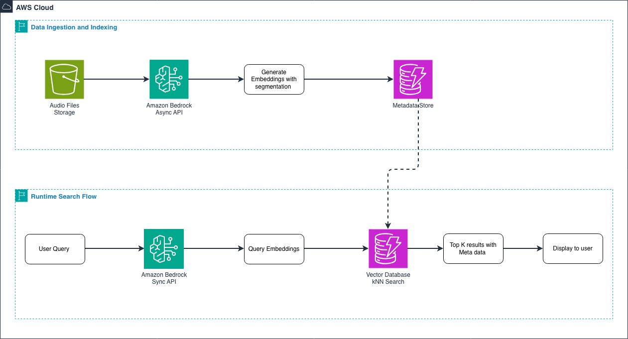
Figure 1 – End-to-end audio embedding workflow

Data ingestion and indexing flow: During the ingestion phase, you process your audio library in bulk. You upload audio files to Amazon S3, then use the asynchronous API to generate embeddings. For long audio files (over 30 seconds), the model automatically segments them into smaller chunks with temporal metadata. You store these embeddings in a vector database along with metadata like filename, duration, and genre. This happens once for your entire audio library.

Runtime search flow: When a user searches, you use the synchronous API to generate an embedding for their query—whether it’s text like “upbeat jazz piano” or another audio clip. Because queries are short, and users expect fast results, the synchronous API provides low-latency responses. The vector database performs a k-NN search to find the most similar audio embeddings, returning results with their associated metadata. This entire search happens in milliseconds.

When you submit audio-only inputs, temporal convolutional networks or transformer-based architectures analyze your acoustic signals for spectro-temporal patterns. Rather than working with raw waveforms, Amazon Nova operates on audio representations like mel-spectrograms or learned audio features, which allows efficient processing of high-sample-rate audio [1].Audio is sequential data that requires temporal context. Your audio segments (up to 30 seconds) pass through architectures with temporal receptive fields that capture acoustic patterns across time [1]. This approach captures rhythm, cadence, prosody, and long-range acoustic dependencies spanning multiple seconds—preserving the full richness of your audio content.

API Operations and Request Structures

When to use synchronous embedding generation: Use the invoke_model API for runtime search when you need embeddings for real-time applications where latency matters [1]. For example, when a user submits a search query, the query text is short, and you want to provide a fast user experience—the synchronous API is ideal for this:

import boto3
import json
 
# Create the Bedrock Runtime client.
bedrock_runtime = boto3.client("bedrock-runtime", region_name="us-east-1")
 
# Define the request body for a search query.
request_body = {
    "taskType": "SINGLE_EMBEDDING",  # Use for single items
    "singleEmbeddingParams": {
        "embeddingPurpose": "GENERIC_RETRIEVAL",  # Use GENERIC_RETRIEVAL for queries
        "embeddingDimension": 1024,  # Choose dimension size
        "text": {
            "truncationMode": "END",  # How to handle long inputs
            "value": "jazz piano music"  # Your search query
        }
    }
}
 
# Invoke the Nova Embeddings model.
response = bedrock_runtime.invoke_model(
    body=json.dumps(request_body),
    modelId="amazon.nova-2-multimodal-embeddings-v1:0",
    contentType="application/json"
)
 
# Extract the embedding from response.
response_body = json.loads(response["body"].read())
embedding = response_body["embeddings"][0]["embedding"]  # float32 array

Understanding request parameters:

• taskType: Choose SINGLE_EMBEDDING for single items or SEGMENTED_EMBEDDING for chunked processing [1, 2]
• embeddingPurpose: Optimizes embeddings for your use case—GENERIC_INDEX for indexing your content, GENERIC_RETRIEVAL for queries, DOCUMENT_RETRIEVAL for document search [1]
• embeddingDimension: Your output dimension choice (3072, 1024, 384, 256) [1]
• truncationMode: How to handle inputs exceeding context length—END truncates at the end, START at beginning [1]

What you get back: The API returns a JSON object containing your embedding:

{
  "embeddings": [
    {
      "embedding": [0.123, -0.456, 0.789, ...],  // float32 array
      "embeddingLength": 1024
    }
  ]
}

When to use asynchronous processing: Amazon Nova Multimodal Embeddings supports two approaches for processing large volumes of content: the asynchronous API and the batch API. Understanding when to use each helps you optimize your workflow.

Asynchronous API: Use the start_async_invoke API when you need to process large individual audio or video files that exceed the synchronous API limits [1]. This is ideal for:

• Processing single large files (multi-hour recordings, full-length videos)
• Files requiring segmentation (over 30 seconds)
• When you need results within hours but not immediately

response = bedrock_runtime.start_async_invoke(
    modelId="amazon.nova-2-multimodal-embeddings-v1:0",
    modelInput=model_input,
    outputDataConfig={
        "s3OutputDataConfig": {"s3Uri": "s3://amzn-s3-demo-bucket/output/"}
    }
)
invocation_arn = response["invocationArn"]
# Poll job status
job = bedrock_runtime.get_async_invoke(invocationArn=invocation_arn)
status = job["status"]  # "InProgress" | "Completed" | "Failed"

When your job completes, it writes output to Amazon S3 in JSONL format (one JSON object per line). For AUDIO_VIDEO_COMBINED mode, you’ll find the output in embedding-audio-video.jsonl [1].

Batch API: Use the batch inference API when you need to process thousands of audio files in a single job [3].

This is ideal for:

• Bulk processing of your entire audio library (thousands to millions of files)
• Cost optimization through batch pricing
• Non-time-sensitive indexing operations where you can wait 24-48 hours
• Processing many small-to-medium sized files efficiently

The batch API offers better cost efficiency for large-scale operations and handles job management automatically. You submit a manifest file with all your input files, and the service processes them in parallel, writing results to S3.

Choosing between async and batch:

• Single large file or real-time segmentation needs? → Use async API
• Thousands of files to process in bulk? → Use batch API
• Need results within hours? → Use async API
• Can wait 24-48 hours for cost savings? → Use batch API

Learn more about batch inference in the Amazon Bedrock batch inference documentation.[3]

Segmentation and Temporal Metadata

Why you need segmentation: If your audio files exceed 30 seconds, you need to segment them [1]. Imagine you have a 2-hour podcast and want to find the specific 30-second segment where the host discusses AI—segmentation makes this possible.

You control chunking with the segmentationConfig parameter:

"segmentationConfig": {
    "durationSeconds": 15  # Generate one embedding every 15 seconds
}
This configuration processes a 5-minute audio file (300 seconds) into 20 segments (300 ÷ 15 = 20), generating 20 embeddings [1]. Each segment receives temporal metadata marking its position in your original file.

Understanding segmented output: The asynchronous API writes your segmented embeddings to JSONL with temporal metadata [1]:

{"startTime": 0.0, "endTime": 15.0, "embedding": [...]}
{"startTime": 15.0, "endTime": 30.0, "embedding": [...]}
{"startTime": 30.0, "endTime": 45.0, "embedding": [...]}

How to parse segmented output:

import json
from boto3 import client
s3 = client("s3", region_name="us-east-1")
# Read JSONL file from S3
response = s3.get_object(Bucket="bucket", Key="output/embedding-audio-video.jsonl")
content = response['Body'].read().decode('utf-8')
segments = []
for line in content.strip().split('n'):
    if line:
        segment = json.loads(line)
        segments.append({
            'start': segment['startTime'],
            'end': segment['endTime'],
            'embedding': segment['embedding'],
            'duration': segment['endTime'] - segment['startTime']
        })
print(f"Processed {len(segments)} segments")
print(f"First segment: {segments[0]['start']:.1f}s - {segments[0]['end']:.1f}s")
print(f"Embedding dimension: {len(segments[0]['embedding'])}")

Real-world use case—temporal search: You can store segmented embeddings with their temporal metadata in a vector database. When someone searches for “customer complaint about billing,” you retrieve the specific 15-second segments with timestamps, giving you precise navigation to relevant moments within multi-hour call recordings. There is no need to listen to the entire recording.

Vector Storage and Indexing Strategies

Referring to the architecture: In Section 2.2, we showed you the end-to-end workflow diagram. Now we’re diving deeper into the Vector Database component—the storage layer where your embeddings live during both the ingestion phase and the runtime search phase. This is the critical component that connects your indexed audio embeddings to fast search queries.

Understanding your storage requirements: Embeddings are float32 arrays requiring 4 bytes per dimension. Here’s what you’ll need:

• 3,072 dimensions: 12,288 bytes (12 KB) per embedding
• 1,024 dimensions: 4,096 bytes (4 KB) per embedding
• 384 dimensions: 1,536 bytes (1.5 KB) per embedding
• 256 dimensions: 1,024 bytes (1 KB) per embedding

Example calculation: For 1 million audio clips with 1,024-dimensional embeddings, you need 4 GB of vector storage (excluding metadata and index structures).

Choosing your dimension size: Larger dimensions give you more detailed representations but require more storage and computation. Smaller dimensions offer a practical balance between retrieval performance and resource efficiency. Start with 1,024 dimensions—it provides excellent accuracy for most applications while keeping costs manageable.

Using Amazon S3 Vectors: You can store and query your embeddings using Amazon S3 Vectors [2]:

s3vectors = boto3.client("s3vectors", region_name="us-east-1")
# Create vector index
s3vectors.create_index(
    vectorBucketName="audio-vectors",
    indexName="audio-embeddings",
    dimension=1024,
    dataType="float32",
    distanceMetric="cosine"
)
# Store embedding with metadata
s3vectors.put_vectors(
    vectorBucketName="audio-vectors",
    indexName="audio-embeddings",
    vectors=[{
        "key": "audio:track_12345",
        "data": {"float32": embedding},
        "metadata": {
            "filename": "track_12345.mp3",
            "duration": 180.5,
            "genre": "jazz",
            "upload_date": "2025-10-28"
        }
    }]
)

How metadata enhances your search: Metadata attributes work alongside embeddings to provide richer search results. When you retrieve results from the vector database, the metadata helps you filter, sort, and display information to users. For example, the genre field lets you filter results to only jazz recordings, duration helps you find tracks within a specific length range, and filename provides the path to the actual audio file for playback. The upload_date can help you prioritize recent content or track data freshness. This combination of semantic similarity (from embeddings) and structured metadata creates a powerful search experience.

Querying your vectors: k-NN search retrieves the top-k most similar vectors [2]:

    vectorBucketName="audio-vectors",
    indexName="audio-embeddings",
    queryVector={"float32": query_embedding},
    topK=10,  # Return 10 most similar results
    returnDistance=True,
    returnMetadata=True
)
for result in response["vectors"]:
    print(f"Key: {result['key']}")
    print(f"Distance: {result['distance']:.4f}")  # Lower = more similar
    print(f"Metadata: {result['metadata']}")
 

Using Amazon OpenSearch Service: OpenSearch provides native k-NN search with HNSW (Hierarchical Navigable Small World) indexes for sub-linear query time complexity [1]. This means your searches stay fast even as your audio library grows to millions of files.

Index configuration:

  "mappings": {
    "properties": {
      "audio_embedding": {
        "type": "knn_vector",
        "dimension": 1024,
        "method": {
          "name": "hnsw",
          "space_type": "cosinesimil",
          "engine": "nmslib",
          "parameters": {"ef_construction": 512, "m": 16}
        }
      },
      "metadata": {"type": "object"}
    }
  }
}

Batch Optimization and Production Patterns

Why batch processing matters: When you process multiple audio files, batch inference improves throughput by reducing network latency overhead [1]. Instead of making separate API calls for each file, you can process them more efficiently.

Example batch pattern:

texts = ["jazz music", "rock music", "classical music"]
vectors = []
for text in texts:
    response = bedrock_runtime.invoke_model(
        body=json.dumps({
            "taskType": "SINGLE_EMBEDDING",
            "singleEmbeddingParams": {
                "embeddingDimension": 1024,
                "text": {"truncationMode": "END", "value": text}
            }
        }),
        modelId="amazon.nova-2-multimodal-embeddings-v1:0",
        contentType="application/json"
    )
    embedding = json.loads(response["body"].read())["embeddings"][0]["embedding"]
    vectors.append(embedding)
# Batch write to vector store
s3vectors.put_vectors(
    vectorBucketName="audio-vectors",
    indexName="audio-embeddings",
    vectors=[
        {"key": f"text:{text}", "data": {"float32": emb}}
        for text, emb in zip(texts, vectors)
    ]
)

Multilingual support: The model supports text inputs in 200+ languages [1]. This supports powerful cross-modal search scenarios: your customers can search in Spanish for audio content indexed in English, or vice versa. The embeddings capture semantic meaning across languages.

Amazon Nova Audio Multimodal Embeddings Deep Dive

Technical Specifications

Model architecture: Amazon Nova Multimodal Embeddings is built on a foundation model trained to understand relationships across different modalities—text, images, documents, video, and audio—within a unified embedding space.

Flexible embedding dimensions: You get four output dimension options: 3,072, 1,024, 384, and 256. Larger dimensions provide more detailed representations but require more storage and computation. Smaller dimensions offer a practical balance between retrieval performance and resource efficiency. This flexibility helps you optimize for your specific application and cost requirements.

Media processing capabilities: For video and audio inputs, the model supports segments of up to 30 seconds, and automatically segments longer files [1]. This segmentation capability is particularly useful when you work with large media files—the model splits them into manageable pieces and creates embeddings for each segment. The output includes embeddings for your video and audio files with temporal metadata.

API flexibility: You can access the model through both synchronous and asynchronous APIs. Use synchronous APIs for querying where latency matters. Use asynchronous APIs for data ingestion and indexing where you can tolerate longer processing times. The asynchronous API supports batch segmentation/chunking for text, audio, and video files. Segmentation refers to splitting a long file into smaller chunks, each of which creates a unique embedding, allowing for fine-grained and more accurate retrieval.

Input methods: You can pass content to embed by specifying an S3 URI or inline as a base64 encoding. This gives you flexibility in how you integrate embeddings into your workflow.

How the workflow works:

1. You use Amazon Nova Multimodal Embeddings to generate embeddings for your video or audio clips
2. You store the embeddings in a vector database
3. When your end-user searches for content, you use Amazon Nova to generate an embedding for their search query
4. Your application compares how similar the search query embedding is to your indexed content embeddings
5. Your application retrieves the content that best matches the search query based on a similarity metric (such as cosine similarity)
6. You show the corresponding content to your end-user

Supported inputs: Your inputs to generate embeddings can be in text, image, document image, video, or audio form. The inputs refer to both the items you use to create the index and the end-user search queries. The model outputs embeddings which you use to retrieve the assets that best match the query to display to your end-user.

Audio format support: Amazon Nova Multimodal Embedding currently supports mp3, wav, and ogg as input formats. These formats cover most common audio use cases from music to speech recordings.

Key Capabilities

Audio-to-Audio search: Find acoustically similar content in your library. For example, find all recordings with similar musical characteristics or speaking styles.

Text-to-Audio search: Use natural language queries to retrieve relevant audio segments. Search for “upbeat jazz piano” or “customer expressing frustration” and get back matching audio clips.

Cross-modal retrieval: Search across images, audio, video, and text simultaneously. This unified approach means you can use one query to search your entire content library regardless of format.

Temporal understanding: The model recognizes actions and events within audio over time. This lets you search for specific moments within long recordings.

When to Choose Amazon Nova

Amazon Nova Multimodal Embeddings is designed for production applications requiring scalable performance, rapid deployment, and minimal operational overhead.

Why choose Amazon Nova:

• Speed to market: Deploy in hours or days, not months
• Managed service: No infrastructure to maintain or models to train
• Cross-modal capabilities: One model for all your content types with enterprise level deployment support
• Continuous improvements: Benefit from model updates without migration work

Decision factors to consider:

• Scale requirements: How many audio files and queries do you need to handle
• Time-to-market: How quickly do you need a working solution
• Expertise availability: Do you have engineering team to maintain custom models
• Integration needs: Do you need seamless AWS service integration

Core application domains: Amazon Nova Multimodal Embeddings serves a wide range of applications optimized for multimodal RAG, semantic search, and clustering:

• Agentic Retrieval-Augmented Generation (RAG): You can use Amazon Nova Multimodal Embeddings for RAG-based applications where the model serves as the embedding for the retrieval task. Your input can be text from documents, images, or document images that interleave text with infographics, video, and audio. The embedding lets you retrieve the most relevant information from your knowledge base that you can provide to an LLM system for improved responses.
• Semantic Search: You can generate embeddings from text, images, document images, video, and audio to power search applications stored in a vector index. A vector index is a specialized embedding space that reduces the number of comparisons needed to return effective results. Because the model captures the nuance of your user’s query within the embedding, it supports advanced search queries that don’t rely on keyword matching. Your users can search for concepts, not just exact words.
• Clustering: You can use Amazon Nova Multimodal Embeddings to generate embeddings from text, images, document images, video, and audio. Clustering algorithms can group together items that are close to each other based on distance or similarity. For example, if you work in media management and want to categorize your media assets across similar themes, you can use the embeddings to cluster similar assets together without needing metadata for each asset. The model understands content similarity automatically.

Conclusion

In this post, we explored how Amazon Nova Multimodal Embeddings enables semantic audio understanding beyond traditional text-based approaches. By representing audio as high-dimensional vectors that capture both acoustic and semantic properties, you can build search systems that understand tone, emotion, and context not just spoken words. We covered the end-to-end workflow for building an audio search system, including:- Generating embeddings using synchronous and asynchronous APIs- Segmenting long audio files with temporal metadata- Storing embeddings in a vector database- Performing k-NN search to retrieve relevant audio segments. This approach allows you to transform large audio libraries into searchable, intelligent datasets that support use cases such as call center analysis, media search, and content discovery.

In our implementation, we took a real-world scenario embedding call center recordings and used Amazon Nova Multimodal Embeddings model to make them searchable by both sentiment and content. Instead of manually tagging calls, we used text queries such as: “Find a call where the speaker sounds angry” or “Show me a conversation about billing issues.” It worked, pulling out the right audio clips on demand. In other words, we turned audio archives into a searchable experience by both tone and topic without the hassle. For those who want to dive deeper, you can see our code samples and snippets linked in the final section.

References

[1] Blog on Amazon Nova Multimodal Embeddings

[2] Nova Embeddings

[3] Supported Regions and models for batch inference

---

About the authors